Sampling-Aware Ancestral State Inference

library(saasi)
library(diversitree)
library(ape)
library(phytools)

Introduction

This vignette demonstrates how to use the saasi package for ancestral state reconstruction.

SAASI (Sampling-Aware Ancestral State Inference) is an ancestral state reconstruction method that accounts for variation in sampling rates among locations or traits.

Unlike traditional methods that assume uniform sampling, SAASI explicitly models heterogeneous sampling, leading to ancestral state estimates that take sampling into account.

SAASI is described in Song et al. (2025).

Installation

You can install the development version of saasi from GitHub with:

# install.packages("remotes")
remotes::install_github("MAGPIE-SFU/saasi")

Overview

The saasi function requires three main inputs:

A phylogenetic tree (class phylo) that is:
- Rooted and binary
- Has branch lengths in units of time (all positive)
- Contains tip states (tree$tip.state) with no missing values
SAASI has the function prepare_tree_for_saasi() which can ensure that these conditions are met.
Transition rate matrix Q (class matrix):
- Rates of transition between states
Use estimate_transition_rates() to estimate this matrix.
Birth-death-sampling parameters (class data.frame):
- Speciation rate
- Extinction/removal rate
- Sampling rate
Use estimate_bds_parameters() to estimate the speciation rate and a single, overall sampling rate. The “extinction rate” (in the language of birth-death models) in infectious disease applications is the inverse of the duration of infectiousness, i.e. the rate of leaving the infectious class.

The output is a data frame containing the probability of each state for each internal node of the phylogenetic tree.

Example: Ebola 2013-2016 West African Ebola Epidemic

Read tree and load metadata

For this example, we use data from Nextstrain (Hadfield et al. 2018; Sagulenko, Puller, and Neher 2018): https://nextstrain.org/ebola/ebov-2013?c=country.

tree <- ape::read.tree(system.file("extdata", "nexstrain_ebola_ebov-2013_smaller.nwk", package = "saasi"))
metadata <- readr::read_tsv(system.file("extdata", "nextstrain_ebola_ebov-2013_metadata.tsv", package = "saasi"))
#> Rows: 1493 Columns: 8
#> ── Column specification ────────────────────────────────────────────────────────
#> Delimiter: "\t"
#> chr  (7): strain, country, division, author, author__url, accession, accessi...
#> date (1): date
#> 
#> ℹ Use `spec()` to retrieve the full column specification for this data.
#> ℹ Specify the column types or set `show_col_types = FALSE` to quiet this message.

First, create a data frame containing strains and states. The first column of the data frame should match tree$tip.label, and the second column should contain the state of interest. Users can skip this step if tree$tip.state already exists.

tip_data <- data.frame(
  tip_label = metadata$strain,
  state = metadata$country
)

Modify the tree to be compatible with saasi

Users can apply the function prepare_tree_for_saasi() to make the tree compatible with saasi. To check if the tree is compatible, use the function check_tree_compatibility(). Here, the function will include the tip states (i.e. their location) in the tree as

ebola_tree <- prepare_tree_for_saasi(tree, tip_data)

This tree is a downsampled version of the 2013 Ebola virus tree from nextstrain. There are 193 tips from three countries.

plot_saasi(ebola_tree, saasi_result = NULL, tip_cex = 1, res = 900)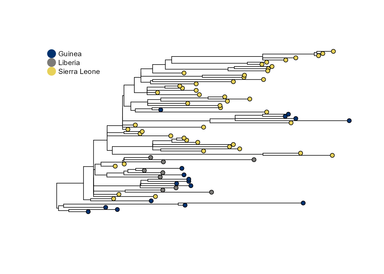

Estimating transition rates

Users can estimate the transition rate matrix Q using the function estimate_transition_rates(). Users can specify the model for the transition rate matrix: 1. Equal rate ER, 2. Symmetric rate SYM, 3. All rates different ARD, and or a custom structure for the matrix.

Q <- estimate_transition_rates(ebola_tree, method = 'fitMk', matrix_structure = 'SYM')

Estimating speciation and sampling rates

Users can estimate speciation and sampling rates using the function estimate_bds_parameters(). In infectious disease applications, users should have some knowledge about the expected removal rate ( $1/\mu$ ) for the disease of interest, as saasi requires the extinction rate as an input (to overcome identifiability limitations). To obtain estimates for the overall speciation and sampling rates, users should have knowledge about the maximum and minimum R0, as well as the upper and lower bounds for the total removal rate $(1/(\mu+\psi))$ .

For Ebola, we assume the total infectious period $(1/(\mu+\psi))$ is between 20 and 40 days. Converting to years, the total removal rate ( $\mu + \psi$ ) is between 9.125 (365/40) and 18.25 (365/20). If we assume $\mu = 5$ , this gives us bounds for the overall sampling rate $\psi$ between 4.125 and 13.25. In this example, we assume R0 is between 1.5 and 3.

rates <- estimate_bds_parameters(
    ebola_tree,
    mu = 5,
    r0_max = 3,
    r0_min = 1.5,
    psi_max = 15,
    infectious_period_min = 20/365, # convert days to years
    infectious_period_max = 40/365, # convert days to years
    n_starts = 100)

Now we set the state-specific sampling and pass the parameters to SAASI. Our overall sampling rate has been estimated (so as to be comparable with $\lambda$ and $\mu$ ); SAASI allows us to account for state-specific relative sampling.

Suppose, for example, that Liberia was known to have sequenced a smaller fraction of the cases than the other states, by a factor of 2.

Setting up input parameters

pars = data.frame(state = colnames(Q), lambda=rates$lambda, mu = rates$mu, psi= rates$psi, row.names = NULL)
pars[(pars$state=="Liberia"),"psi"] = pars[(pars$state=="Liberia"), "psi"]/2 # set sampling rate to be 1/2 the baseline

Run saasi analysis

saasi_ebola <- saasi(ebola_tree, Q, pars)
#> Tree is compatible with SAASI

Plot and save the result

Users can use the built-in function plot_saasi() to visualize results.

p1 <- plot_saasi(ebola_tree, saasi_ebola, tip_cex = 1, node_cex = 0.5, res = 900)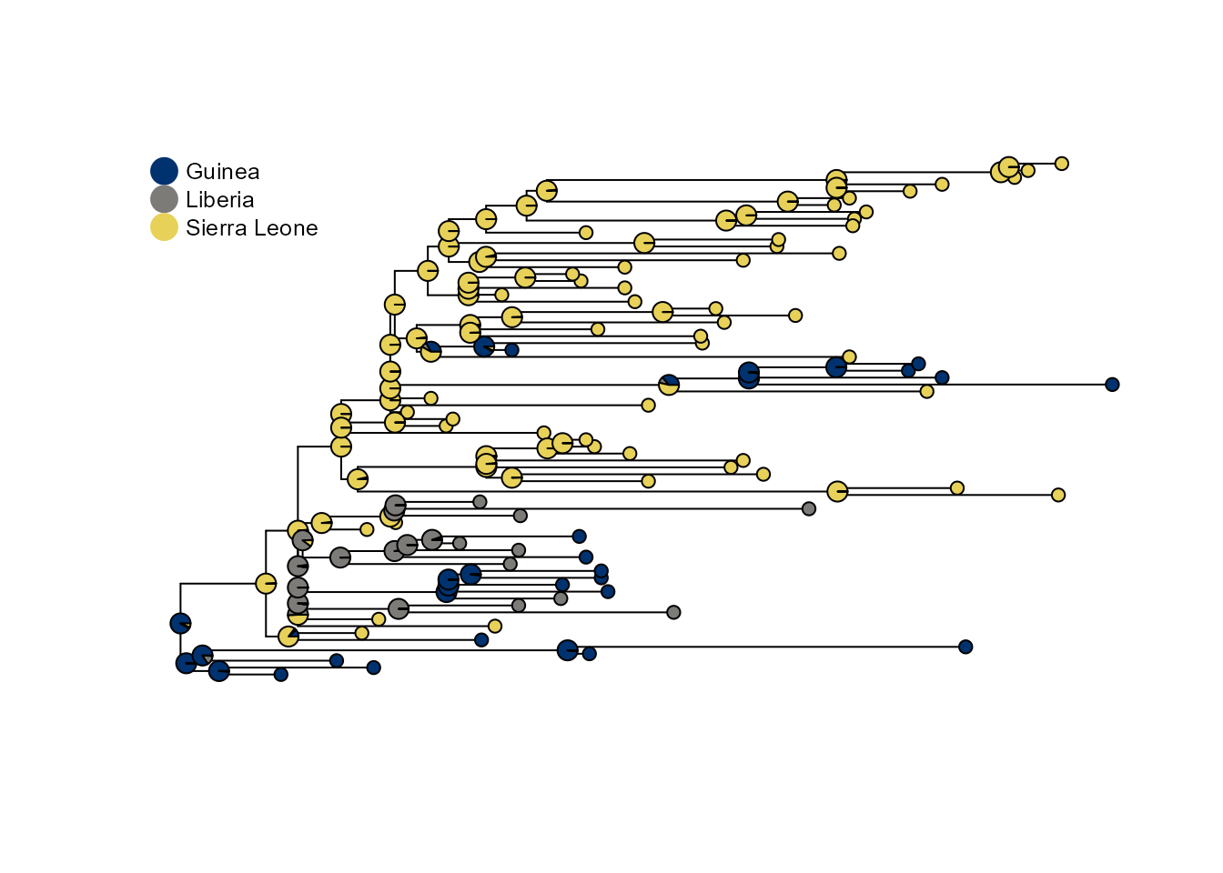

Compare to equal sampling

If all states had comparable sampling we would obtain a different ancestral state reconstruction:

pars = data.frame(state = colnames(Q), lambda=rates$lambda, mu = rates$mu, psi= rates$psi, row.names = NULL)
saasi_ebola2 <- saasi(ebola_tree, Q, pars)
#> Tree is compatible with SAASI

p2 <- plot_saasi(ebola_tree, saasi_ebola2, tip_cex = 1, node_cex = 0.5, res = 900)

Interpreting results

The saasi() function returns a data frame with probability distributions over states for each internal node. Higher probabilities indicate greater confidence in that ancestral state. In this example, if we assume that Liberia has sampled at a lower rate than the other two countries, we see more internal nodes inferred to be in Liberia than if its sampling is the same as the other locations. This is because SAASI accounts for undetected cases in Liberia.

Note that Liberia and the factor of 2 are chosen entirely at random for the purposes of this vignette and do not represent any knowledge or opinion of the authors about the relative sampling during this outbreak.

Hadfield, James, Colin Megill, Sidney M Bell, John Huddleston, Barney Potter, Charlton Callender, Pavel Sagulenko, Trevor Bedford, and Richard A Neher. 2018. “Nextstrain: Real-Time Tracking of Pathogen Evolution.” Bioinformatics 34 (23): 4121–23. https://doi.org/10.1093/bioinformatics/bty407.

Sagulenko, Pavel, Vadim Puller, and Richard A Neher. 2018. “TreeTime: Maximum-Likelihood Phylodynamic Analysis.” Virus Evol. 4 (1). https://doi.org/10.1093/ve/vex042.

Song, Yexuan, Ivan Gill, Ailene MacPherson, and Caroline Colijn. 2025. “Sampling Aware Ancestral State Inference.” bioRxiv, 2025–05. https://doi.org/10.1101/2025.05.20.655151.

Yexuan Song, Caroline Colijn

2026-03-06